Episode 6 in this series on principles to follow when ranking environmental projects. A factor that influences the level of benefits from many environmental projects is the extent to which people cooperate with the project by adopting new behaviours or practices. 

In PDs 237, 238 and 239 I talked about estimating the benefits of environmental projects, as part of the process of ranking projects. To keep things simple, I focused on the predicted environmental changes and their values, but there are other benefit-related factors that we need to account for too. The first of these is human behaviour.

Often, the success of a project depends on the behaviour of certain people. For example, the aim of the project might be to reduce eutrophication in an urban river by having people reduce their use of fertilizers in home gardens, or to reduce air pollution by having factories install systems to remove pollutants from chimney emissions.

The issue is that, typically, not everybody cooperates with these sorts of projects. The degree of compliance varies from project to project, and this needs to be accounted for when we rank projects. Otherwise we risk giving funds to projects that have great potential but little benefit in practice.

Later on I’ll discuss the estimation of adoption/compliance for particular projects. First I want to talk about how this information should be included in the project-ranking process.

To start with, define A as the level of adoption/compliance as a proportion of the level needed to achieve the project’s goal. If A = 0.5, that means that compliance was only half the level we would have needed.

Usually, if A is less than 1.0, it doesn’t mean the project generates no benefits. There is some relationship between A and the benefits generated. Figure 6 shows one possible example, where proportional benefits [f(A)] increase slowly at low levels of adoption, then rapidly for a while, before flattening off again at high adoption. Other shapes are possible, but whatever the shape is, we know these important facts about it: it must range from zero (no adoption, so no project benefits) up to 1.0 (full adoption, so full project benefits). This follows from the fact that we define f(A) as the proportion of target project benefits achieved.

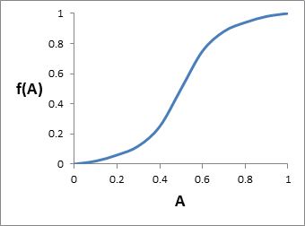
Figure 6.

This makes it obvious how f(A) should be included in the formula we use for ranking projects: it should be multiplied by the potential benefits.

Benefit = [V(P₁) – V(P₀)] × f(A)

The terms in square brackets represent the difference in values between P₁ (physical condition with the project) and P₀ (physical condition without the project), assuming that there is full compliance, and this is scaled down by f(A) to reflect the effect of less-than-full compliance. In other words, [V(P₁) – V(P₀)] represents potential benefits, and we scale that down by f(A) to get actual benefits – actual in the sense of accounting for lower adoption. (Equivalently, using the approach outlined in PD239, Benefit = V(P’) × W × f(A).)

[Note that if a project does not require anybody to change their behaviour, you would set f(A) = 1.]

This formula demonstrates an important principle for the ranking formula: if the benefits are proportional to a variable (as they are for f(A)), then that variable must be multiplied by the rest of the equation for benefits. Only that way can the formula correctly represent the reality that, if the variable is zero, the benefits must be zero, and if the variable is at its maximum value, so too are the benefits. As a way of testing whether this is relevant, ask this question: if the variable was zero, would the overall benefits be zero? If the answer is yes, the variable should probably be multiplied.

Unfortunately, a common way that people combine variables like these in the ranking formula is to give them weights (meant to reflect their relative importance) and add them up, something like this:

Benefit = z₁ × [V(P₁) – V(P₀)] + z₂ × f(A)

where z₁ and z₂ are the weights. This is a bad mistake. With this formula, it is impossible to specify any set of weights that will make it represent the reality that the benefits are proportional to f(A). Experiments I’ve done with this formula show that it can result in wildly inaccurate project rankings, leading to a big loss of environmental values. Switching from this bad formula to the correct one can be like doubling the program budget (in terms of the extra benefits generated) (see PD158).

On the other hand, a simplification that is probably reasonable is to approximate f(A) by a straight line. In practice, we usually have too little information about the actual shape of f(A) in specific cases to be able to argue that its shape should be non-linear, and even if it is, it’s unlikely to be so non-linear that an assumption of linearity would have very bad consequences. If you are comfortable with this approximation, you can just use A in the formula rather than f(A).

Benefit = [V(P₁) – V(P₀)] × A

or

Benefit = V(P’) × W × A

That’s what we usually do in INFFER; in the absence of better information, and in the interests of simplicity, we use A rather than f(A) in the formula. But if somebody did have accurate numbers for f(A), we would use them instead.

Finally, some brief comments on predicting the level of compliance/adoption for a project. There has been a great deal of research into the factors that influence the uptake of new practices (e.g., Rogers 2003; Pannell et al., 2006, and see www.RuralPracticeChange.org), so we have a good understanding of this. There are many different influential factors, and the set of important factors varies substantially from case to case.

However, despite the wealth of research, it remains difficult to make quantitative predictions about compliance for a specific project. One generalisation I would make is that people who develop projects are usually too optimistic about the level and speed of adoption that is realistic to expect – sometimes far too optimistic.

Specific predictions require specific knowledge about the population of potential adopters, and the practice we would like them to adopt. As far as I’m aware, there is only one tool that has been developed to help make quantitative predictions about adoption. This is ADOPT, the Adoption and Diffusion Outcome Prediction Tool. ADOPT is designed for predicting adoption of new practices by farmers. It is not suitable for other contexts, although it might provide insights and understanding that help people to make the required judgments.

Further reading

Pannell, D.J., Marshall, G.R., Barr, N., Curtis, A., Vanclay, F. and Wilkinson, R. (2006). Understanding and promoting adoption of conservation practices by rural landholders. Australian Journal of Experimental Agriculture 46(11): 1407-1424. If you or your organisation subscribes to the Australian Journal of Experimental Agriculture you can access the paper at:http://www.publish.csiro.au/nid/72/paper/EA05037.htm (or non-subscribers can buy a copy on-line for A$25). Otherwise, email David.Pannell@uwa.edu.au to ask for a copy.

Pannell, D.J., Roberts, A.M., Park, G. and Alexander, J. (2013). Designing a practical and rigorous framework for comprehensive evaluation and prioritisation of environmental projects, Wildlife Research 40(2), 126-133. Journal web page ♦ Pre-publication version at IDEAS

Rogers, E.M. (2003). Diffusion of innovations, 5^th ed., Free Press, New York.