Episode 8 in this series on principles to follow when ranking environmental projects. It is about how to account for time when estimating project benefits.  

Different projects involve different time lags until benefits are generated. There are at least four potential causes of lags:

1. Some projects take a significant amount of time to implement (implementation lags). For example, if a project relies on new research being conducted, it could take several years before results are available. Typically, implementation lags for different types of project range from a year to a decade.
2. It may take a while for the physical actions implemented in a project to take effect and to start generating benefits (effect lags). For example, if the project involves planting trees, they take a while to grow. Realistic effect lags in environmental projects range from zero to decades.
3. The project may be addressing a threat which has not occurred yet but is expected to occur in future (threat lag). For example, between 2001 and 2008 the Australian Government invested in many projects that were intended to prevent the occurrence of dryland salinity in rural areas. In some of those areas, salinity was not predicted to occur until several decades in the future. In other cases, the threat lag was zero – the problem was already occurring.
4. If a project requires other people to change their behaviour or management, it may take a while for most people to change (adoption lag). Realistic adoption lags for substantial changes range from around five years (in exceptional cases) to several decades.

Given this variety of lags types, and the range of lag lengths within each lag type, projects vary widely in the overall time lag until benefits are generated. This makes it an important factor to consider when ranking projects but it’s one that is commonly ignored.

Looking ahead from the time when an environmental project is being considered (time zero), a typical pattern of benefits over time (combining all the types of lags) is shown in Figure 7. This project generates half of its benefits by year 18 and 90% by year 25.

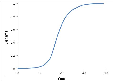
Figure 7.

The question is, how should differences in the overall time lags for different projects influence their rankings? Here’s a simple example to illustrate how to think about it. (Inflation has been factored out of all the numbers in this example.)

Suppose there are two projects to rank. Both of them would involve costs of $1 million in 2014 and both generate benefits worth $2 million in the future. In one project, the $2m benefits would be delivered in 2018 while in the other, the benefits would occur in 2033. The $1m in 2014 has to be borrowed (at an interest rate of 5%) and will be repaid in full, including interest, when the benefits are generated. Thus, for the quick project, in 2018 we face a benefit (the $2m) and a cost equal to the repayment. Similarly, for the slow project, in 2033 there is a benefit of $2m and a different repayment cost. How do the costs and benefits stack up in each case?

The repayment cost would be calculated as follows:

Future repayment = Present cost × (1 + r)^L

where Present cost is the amount borrowed up front, r is the interest rate (assumed to be 5%, after taking out inflation) and L is the time lag until the loan has to be repaid.

Compounding the interest costs over four years, the total repayment in 2018 would be $1.22 m. This is less than the $2 m benefit, so the quick project has a positive net benefit of $0.78 m in 2018. On the other hand, by 2033, the repayment would by $2.57 m, so the cost of the slow project would be greater than the benefit generated. Clearly, the quicker project would be preferred.

The same logic applies even if the money used to pay for the project doesn’t have to be borrowed. The money used has an ‘opportunity cost’ (you miss out on the benefits of investing it in some other way) and that cost compounds over time in the same way as the interest on a loan.

The way that economists usually apply this thinking is to use the present as the reference date. Instead of compounding present costs into the future, they discount future benefits (and costs) back to the present. It amounts to exactly the same thing when it comes to ranking projects, and it has the advantage that it is easy to compare discounted values to the current value of money. The formula for present values is just the reverse of the repayment formula:

Present value = Future value / (1 + r)^L

Some people object to the idea of discounting future benefits, arguing that it is, in some sense, unfair or unreasonable. What they don’t realise is that it’s not really about the benefits – it’s about the costs. Interest costs (or other opportunity costs) are real costs and shouldn’t be ignored, but that’s what you would be doing if you refused to discount benefits.

It’s true that discounting benefits and costs in the distant future (e.g. 100 years) is more complicated, as issues of high uncertainty and inter-generational equity become important (e.g. see PD34), but for shorter time frames (up to say 30 years) the logic behind discounting is robust (PD224). A 5% real discount rate (with inflation factored out) is a pretty good general-purpose discount rate that’s suitable for many environmental projects.

In principle, if we knew the year-by-year pattern of benefits (like in Figure 7), we would discount the benefit for each year and add them up to get the total present value of benefits. That would be the measure of benefits we used in the top line of the Benefit: Cost Ratio. If you have the required information, this is simple to do. Of course, getting the required information might not be simple.

In practice, there is usually a lot of uncertainty about how the benefits will play out over time. Recognising that uncertainty, it is probably usually not worth being too precise about the shape of the curve. A highly simplified curve, like the one in Figure 8, might be sufficient. All you need to know to specify this curve is the peak level of benefits (corresponding to the plateau in Figure 7), and the year when it will be achieved (corresponding to the year in Figure 7 when most of the benefits would be achieved).

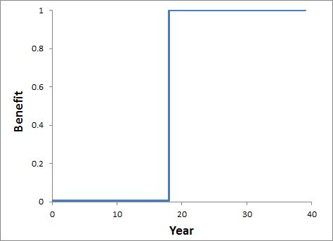
Figure 8.

This benefit curve is based on another convenient assumption: that the benefits, once, generated, will last forever. This is not too unreasonable if allowance is made for long-term maintenance funding (see PD241 on project risks and a later post on project costs).

The simplified benefit curve has an advantage when it comes to calculating the present value of benefits. Rather than having to discount the benefits separately for each year (which is required if using Figure 7), we can just discount one number: the change in environmental values resulting from the project.

Benefit = [V(P₁) – V(P₀)] / (1+r)^L

This works because the overall value of the environmental asset (V(P)) consists of the discounted sum of its future benefits. So, looking at Figure 8, the change in value at year 18 consists of the discounted sum of benefits in all subsequent years. To convert that into a present value, we just need to discount them for another 18 years, which is what the above equation does if we set L = 18.

As discussed in previous posts, we also need to allow for adoption/compliance and project risks, so the equation for expected benefit is:

Expected benefit = [V(P₁) – V(P₀)] × A × (1 – R) / (1+r)^L

or

Expected benefit = V(P’) × W × A × (1 – R) / (1+r)^L

[I have combined the various project risks into one variable, R, to stop the equation getting too ugly. See PD241.]

The time lag until benefits, L (=18 in Figure 8) links back to the earlier post about measuring benefits as the difference in environmental value with and without the project (PD237). In that post I noted that,

A practical simplification is to estimate the environmental benefits based on the difference in the asset value with and without the project in a particular future year. For example, we might choose to focus on 25 years in the future, and estimate values at that date with and without the project.

The selection of L tells us which particular future year to use for this with-vs-without comparison. So, for the example in Figure 8, the difference in values with and without the project would be estimated for year 18.

In PD239 I discussed several possible ways to estimate and represent environmental values, some of which didn’t involve expressing values in dollars (or Euros or Pounds or whatever). It might seem that discounting is not relevant to non-dollar values, but it is. Remember that discounting is used to account for the fact that an up-front cost grows over time due to compounded interest costs (or other opportunity costs), so it is applicable to any logical and consistent quantitative method for expressing future benefits. When comparing future benefits that occur at different times, you need to account for interest accumulating on up-front costs, even if the future benefits are not expressed in dollars. So you need to discount.

Further reading

Pannell, D.J., Roberts, A.M., Park, G. and Alexander, J. (2013). Designing a practical and rigorous framework for comprehensive evaluation and prioritisation of environmental projects, Wildlife Research 40(2), 126-133. Journal web page ♦ Pre-publication version at IDEAS